Differential Equations

Second Order Equations

2nd Order Diff Equations Logo

Newton’s Second Law of Motion

Solved Problems

Example 1.

A body begins to fall from a height \(H\) under the action of gravity. While falling it experiences resistance proportional to the velocity. Determine the time of the drop.

Solution.

There are two forces acting on the body (Figure
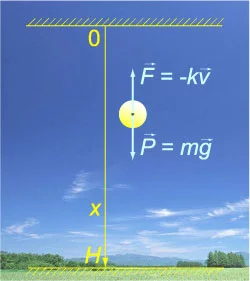
 \(1\)): the force of gravity \(P = mg\) and the drag force \(F = -kv.\)

Two forces acting on the body: the force of gravity and the drag force
Figure 1.

We direct the \(x\)-axis vertically downwards. We assume that the initial coordinate is \(x = 0\) and it is equal to \(x = H\) when the body hits the ground.

Considering the projection on the \(x\)-axis the dynamics equation can be written as

\[m\frac{{{d^2}x}}{{d{t^2}}} = mg - k\frac{{dx}}{{dt}}.\]

This problem is a variation of Case \(2,\) when the force depends on the velocity.

First we find the velocity \({v\left( t \right)}\) from the equation

\[m\frac{{dv}}{{dt}} = mg - kv,\;\; \Rightarrow \frac{{dv}}{{dt}} = g - \frac{k}{m}v.\]

Separating the variables, we have

\[\frac{{dv}}{{g - \frac{k}{m}v}} = dt,\;\; \Rightarrow \int\limits_0^v {\frac{{du}}{{g - \frac{k}{m}u}}} = t.\]

Here, \(v\) is the velocity at time \(t,\) \(u\) is the variable of integration. The solution is as follows:

\[- \frac{m}{k}\int\limits_0^v {\frac{{d\left( {g - \frac{k}{m}u} \right)}}{{g - \frac{k}{m}u}}} = t,\;\; \Rightarrow - \frac{m}{k}\left. {\left[ {\ln \left( {g - \frac{k}{m}u} \right)} \right]} \right|_0^v = t,\;\; \Rightarrow \ln \frac{{g - \frac{k}{m}u}}{g} = - \frac{k}{m}t,\;\; \Rightarrow \ln \left( {1 - \frac{k}{{mg}}v} \right) = - \frac{k}{m}t,\;\; \Rightarrow 1 - \frac{k}{{mg}}v = {e^{ - {\frac{k}{m}} t}},\;\; \Rightarrow \frac{k}{{mg}}v = 1 - {e^{ - {\frac{k}{m}} t}},\;\; \Rightarrow v\left( t \right) = \frac{{mg}}{k}\left( {1 - {e^{ - {\frac{k}{m}} t}}} \right).\]

We integrate again:

\[x\left( t \right) = \frac{{mg}}{k}\int\limits_0^t {\left( {1 - {e^{ - {\frac{k}{m}} \tau }}} \right)d\tau } = \frac{{mg}}{k}\left[ {\left( {t + \frac{m}{k}{e^{ - {\frac{k}{m}} t}}} \right) - \left( {0 + \frac{m}{k}{e^{ - {\frac{k}{m}}0}}} \right)} \right] = \frac{{mg}}{k}\left[ {t - \frac{m}{k}\left( {1 - {e^{ - {\frac{k}{m}} t}}} \right)} \right].\]

Assume that the body reaches the Earth's surface at \(t = T\) when it traverses the distance \(x = H.\) As it can be seen, the time \(T\) is given by the implicit algebraic equation

\[H = \frac{{mg}}{k}\left[ {T - \frac{m}{k}\left( {1 - {e^{ - {\frac{k}{m}}T}}} \right)} \right].\]

The value of \(T\) can be estimated approximately, given that the term \({{e^{ - {\frac{k}{m}} T}}}\) approaches zero for large \(T.\) Then

\[H \approx \frac{{mg}}{k}\left( {T - \frac{m}{k}} \right)\;\; \text{or}\;\;T\left( H \right) \approx \frac{{kH}}{{mg}} + \frac{m}{k}.\]

The resulting approximate dependence of \(T\left( H \right)\) is linear, which corresponds to the uniform motion of the body. Its curve (for \(m = 1\;\text{kg},\) \(k = 1\;\text{N} \cdot {\frac{\text{s}}{\text{m}}}\)) is shown in Figure \(2\) (the red line \(3\)). For comparison, the graph shows two other curves \(T\left( H \right)\) describing:

Falling time T depending on Height H in various approximations
Figure 2.

It is seen from these graphs that the air resistance force compensates the force of gravity in a few seconds after the start of the drop. After that, the motion of the body becomes uniform. Therefore, when falling from a large height (in this example, more than \(20\;\text{m}\)), one can use the approximate formula for \(T\left( H \right)\) to estimate the falling time.

Example 2.

At the initial moment, a chain of length \(L\) hangs over the edge of the table so that the force of gravity is balanced by the friction force (Figure \(3\)). As a result of a small shift \(\varepsilon\) the chain starts sliding. Determine the time \(T,\) for which the chain completely slips off the table. The coefficient of friction between the chain and the surface of the table is equal to \(\mu.\)

Solution.

The movement of chain and forces acting on it
Figure 3.

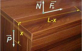
The movement of the chain is completely determined by two variable forces:

According to Newton's second law, the differential equation of motion of the chain has the form:

\[m\frac{{{d^2}x}}{{d{t^2}}} = P - {F_{\text{fr}}},\;\; \Rightarrow m\frac{{{d^2}x}}{{d{t^2}}} = mg\frac{x}{L} - \mu mg\frac{{L - x}}{L},\;\; \Rightarrow \frac{{{d^2}x}}{{d{t^2}}} = g\frac{x}{L} - \mu g\frac{{L - x}}{L},\;\; \Rightarrow \frac{{{d^2}x}}{{d{t^2}}} - \frac{{\left( {1 + \mu } \right)g}}{L}x = - \mu g.\]

We got a second order nonhomogeneous differential equation with constant coefficients. Let us solve this equation. First we consider the associated homogeneous equation:

\[\frac{{{d^2}x}}{{d{t^2}}} - \frac{{\left( {1 + \mu } \right)g}}{L}x = 0.\]

The roots of the characteristic equation have the following values:

\[{n^2} - \frac{{\left( {1 + \mu } \right)g}}{L} = 0,\;\; \Rightarrow {n_{1,2}} = \pm \sqrt {\frac{{\left( {1 + \mu } \right)g}}{L}} .\]

Then the general solution of the homogeneous equation can be written as

\[{x_0} = {C_1}{e^{\sqrt {\frac{{\left( {1 + \mu } \right)g}}{L}} t}} + {C_2}{e^{ - \sqrt {\frac{{\left( {1 + \mu } \right)g}}{L}} t}}.\]

We define the constants \({C_1}, {C_2}\) later using the initial conditions.

We now construct a particular solution of the nonhomogeneous equation. The right side is a constant expression, so we seek a particular solution in the form of a constant number: \({x_1} = A.\) Substituting \({x_1} = A,\) \({x^{\prime\prime}_1} = 0\) in the original equation, we obtain:

\[0 - \frac{{\left( {1 + \mu } \right)g}}{L}A = - \mu g,\;\; \Rightarrow A = \frac{{\mu \cancel{g}L}}{{\left( {1 + \mu } \right)\cancel{g}}} = \frac{{\mu L}}{{1 + \mu }}.\]

Thus, the general solution of the inhomogeneous equation has the form:

\[x = {x_0} + {x_1} = {C_1}{e^{\sqrt {\frac{{\left( {1 + \mu } \right)g}}{L}} t}} + {C_2}{e^{ - \sqrt {\frac{{\left( {1 + \mu } \right)g}}{L}} t}} + \frac{{\mu L}}{{1 + \mu }}.\]

Consider the initial conditions and determine the coefficients \({C_1}\) and \({C_2}.\) As the chain was in equilibrium, the following equation is valid:

\[P = {F_{\text{fr}}},\;\; \Rightarrow mg\frac{x}{L} = \mu mg\frac{{L - x}}{L}.\]

It follows that the length of the hanging part of the chain at equilibrium is

\[x = \frac{{\mu L}}{{1 + \mu }}.\]

By the condition of the problem, at the initial time the chain gets an additional shift \(\varepsilon,\) so that the initial conditions are written as

\[\left\{ \begin{array}{l} x\left( {t = 0} \right) = \frac{{\mu L}}{{1 + \mu }} + \varepsilon \\ v\left( {t = 0} \right) = 0 \end{array} \right..\]

Now we can calculate the coefficients \({C_1}\) and \({C_2}:\)

\[\left\{ \begin{array}{l} {{C_1} \cdot 1 + {C_2} \cdot 1 + \cancel{\frac{{\mu L}}{{1 + \mu }}} = \cancel{\frac{{\mu L}}{{1 + \mu }}} + \varepsilon }\\ {{C_1} \cdot \sqrt {\frac{{\left( {1 + \mu } \right)g}}{L}} - {C_2} \cdot \sqrt {\frac{{\left( {1 + \mu } \right)g}}{L}} } ={ 0} \end{array} \right.,\;\; \Rightarrow \left\{ \begin{array}{l} {C_1} + {C_2} = \varepsilon \\ {C_1} - {C_2} = 0 \end{array} \right.,\;\; \Rightarrow {C_1} = {C_2} = \frac{\varepsilon }{2}.\]

Hence, the sliding of the chain is described by

\[x\left( t \right) = \frac{\varepsilon }{2}{e^{\sqrt {\frac{{\left( {1 + \mu } \right)g}}{L}} t}} + \frac{\varepsilon }{2}{e^{ - \sqrt {\frac{{\left( {1 + \mu } \right)g}}{L}} t}} + \frac{{\mu L}}{{1 + \mu }}.\]

The chain slips off the table at time \(T,\) where \(x\left( T \right) = L.\) As a result, we have the following algebraic equation for \(T:\)

\[\frac{\varepsilon }{2}{e^{\sqrt {\frac{{\left( {1 + \mu } \right)g}}{L}} T}} + \frac{\varepsilon }{2}{e^{ - \sqrt {\frac{{\left( {1 + \mu } \right)g}}{L}} T}} + \frac{{\mu L}}{{1 + \mu }} = L.\]

The expression for \(T\) can be written explicitly. To do this, we multiply the equation by \({e^{\sqrt {\frac{{\left( {1 + \mu } \right)g}}{L}} T}}:\)

\[\frac{\varepsilon }{2}{e^{2\sqrt {\frac{{\left( {1 + \mu } \right)g}}{L}} T}} - \frac{L}{{1 + \mu }}{e^{\sqrt {\frac{{\left( {1 + \mu } \right)g}}{L}} T}} + \frac{\varepsilon }{2} = 0.\]

Denoting \(z = {e^{\sqrt {\frac{{\left( {1 + \mu } \right)g}}{L}} T}},\) we obtain the quadratic equation:

\[\varepsilon {z^2} - \frac{{2L}}{{1 + \mu }}z + \varepsilon = 0,\;\; \Rightarrow D = \frac{{4{L^2}}}{{{{\left( {1 + \mu } \right)}^2}}} - 4{\varepsilon ^2},\;\; \Rightarrow {z_{1,2}} = \frac{{\frac{{2L}}{{1 + \mu }} \pm \sqrt {\frac{{4{L^2}}}{{{{\left( {1 + \mu } \right)}^2}}} - 4{\varepsilon ^2}} }}{{2\varepsilon }} = \frac{L}{{\left( {1 + \mu } \right)\varepsilon }} \pm \sqrt {\frac{{{L^2}}}{{{{\left( {1 + \mu } \right)}^2}{\varepsilon ^2}}} - 1} .\]

Here we only take the root with \(+\) sign to satisfy the inequality

\[e^{\sqrt {\frac{{\left( {1 + \mu } \right)g}}{L}} T} \gt e^{ - \sqrt {\frac{{\left( {1 + \mu } \right)g}}{L}} T}.\]

Hence, the solution is given by

\[{e^{\sqrt {\frac{{\left( {1 + \mu } \right)g}}{L}} T}} = \frac{L}{{\left( {1 + \mu } \right)\varepsilon }} + \sqrt {\frac{{{L^2}}}{{{{\left( {1 + \mu } \right)}^2}{\varepsilon ^2}}} - 1} , \;\;\Rightarrow T = \sqrt {\frac{L}{{\left( {1 + \mu } \right)g}}} \ln \left[ {\frac{L}{{\left( {1 + \mu } \right)\varepsilon }} + \sqrt {\frac{{{L^2}}}{{{{\left( {1 + \mu } \right)}^2}{\varepsilon ^2}}} - 1} } \right].\]

Interestingly, the time of sliding \(T\) in this model depends essentially on the initial displacement \(\varepsilon\) with respect to the equilibrium position. As \(\varepsilon \to 0,\) we formally get \(T \to \infty.\) Dependence of the time of sliding \(T\) on the displacement \(\varepsilon\) for chains of different lengths \(L\) is shown above in Figure \(4.\)

Sliding time depending on the initial displacement
Figure 4.
Page 1 Page 2