
Equation of Catenary
Solved Problems
Example 1.
Determine the shape of the cable supporting a suspension bridge.
Solution.
This problem is similar to the problem considered above. The only difference is that the force of gravity acting on an element of the cable is not proportional to its length \(\Delta s,\) but will be equal to the weight of the corresponding section of the bridge of the length \(\Delta s,\) that is
where \(\mu\) is a coefficient of proportionality.
Then the equilibrium condition for a differential element of the cable \(ds\) can be written in the form
Integrating the simple differential equation twice, we find the shape of the cable:
where \({C_1},{C_2}\) are constants of integration depending on the initial conditions.
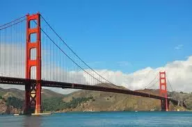
Thus, the cable of a suspension bridge takes the form not of a catenary, but a parabola. So, for example, the suspension cables of the Golden Gate Bridge in San Francisco look like a parabola (Figure \(5\)).
Example 2.
Determine the shape of a nonuniform catenary of equal strength.
Solution.
Let the cable has a variable thickness, which varies so that the stress in any section (and thus the resistance to tearing) remains the same. This cable has a maximum thickness at the points of suspension and a minimum thickness at the bottom.
In this case the conditions of equilibrium of an arbitrary element of the cable (see Figure \(2\) on the previous page) are written as
Here \({T_0}\) denotes the horizontal component of the tension force, \(\alpha\) is the angle between the tangent to the catenary and the \(x\)-axis, \(\rho\) is the density of the catenary material, \(g\) is the acceleration of gravity, \({A\left( s \right)}\) is the cross sectional area of the cable, which is a variable in the given example.
We can express \(T\) from the first equation:
Substituting into the second equation gives:
Take into account that \(\tan\alpha = \frac{{dy}}{{dx}} = y'.\) Therefore one can write:
As the strength \(\sigma\) is equal to \(\sigma = \frac{T}{A},\) we can substitute the expression \(A = \frac{T}{\sigma } = \frac{{{T_0}}}{{\sigma \cos \alpha }}\) in the right side of the equation. Then the equation becomes
By the condition of the problem, the strength \(\sigma\) is a constant for all cross sections. Therefore we take \(\sigma\) out of the integral sign.
Differentiate both sides with respect to the variable \(s:\)
Since \(\cos \alpha = \frac{{dx}}{{ds}},\) we get the following differential equation:
This is a differential equation of kind \(F\left( {y',y^{\prime\prime}} \right) = 0,\) describing the shape of a catenary of equal strength. It can be easily integrated by separating variables:
Using the initial condition \(y'\left( {x = 0} \right) = 0\) we find that the constant \({C_1}\) is zero. Therefore
Integrate once more:
The constant \({C_2}\) can be set to \(0\) after choosing the appropriate coordinate system.
Thus, the shape of the catenary of equal strength is given by the function
where \(b\) denotes \(\frac{{\rho g}}{\sigma }.\) The graph of this function for different values of \(b\) is shown in Figure \(6.\)
